Stay tuned for future updates!
Vehicle Bicycle Model

Kinematic Models: Kinematic models are simplifications of dynamic models that ignore tire forces, gravity, and mass. This simplification reduces the accuracy of the models, but it also makes them more tractable. At low and moderate speeds, kinematic models often approximate the actual vehicle dynamics.
Dynamic Models: Dynamic models aim to embody the actual vehicle dynamics as closely as possible. They might encompass tire forces, longitudinal and lateral forces, inertia, gravity, air resistance, drag, mass, and the geometry of the vehicle. Not all dynamic models are created equal. Some may consider more of these factors than others. Advanced dynamic models even take internal vehicle forces into account. For example, how responsive the chassis suspension is.
Reference Trajectory: The reference trajectory is typically passed to the control block as a polynomial. This polynomial is usually 3rd order, since third order polynomials will fit trajectories for most roads. We need to fit 3rd order polynomials to waypoints (x, y) in C++ using Eigen, and evaluate the output.
Pure Pursuit Lateral Controller (Kinematic Bicycle Model)
Pure Pursuit Geometry
\(\theta\): heading of vehicle or yaw angle of vehicle
\(\dot{\theta}\): rotation rate of vehicle or yaw rate of vehicle
\(\delta_f\): front steering angle
\(L\): wheelbase
\(l_d\): look-ahead distance
\(\alpha\): angle between the vehicle’s heading vector and the look-ahead vector
\(e_{l_d}\): crosstrack error, \(e_{l_d}(t) = l_d sin(\alpha(t))\)
\(\kappa\): path curvature
\(v_x\): vehicle speed in the direction of its x-axis
\(k_{dd}\): gain of pure pursuit controller, \(l_d = k_{dd}v_x(t)\)
$$\delta_f(t) = tan^{-1}(\frac{2Lsin(\alpha(t))}{l_d}) = tan^{-1}(\frac{2Lsin(\alpha(t))}{k_{dd}v_x(t)})$$
$$\delta_f(t) = tan^{-1}(\frac{2L}{l^2_d}e_{l_d}(t))$$
Pure pursuit controller is a proportional controller of the front steering angle \(\delta_f\) operating on a crosstrack error \(e_{l_d}\) with some look-ahead distance \(l_d\) in front of the vehicle and having a gain of \(2L/l^2_d\).
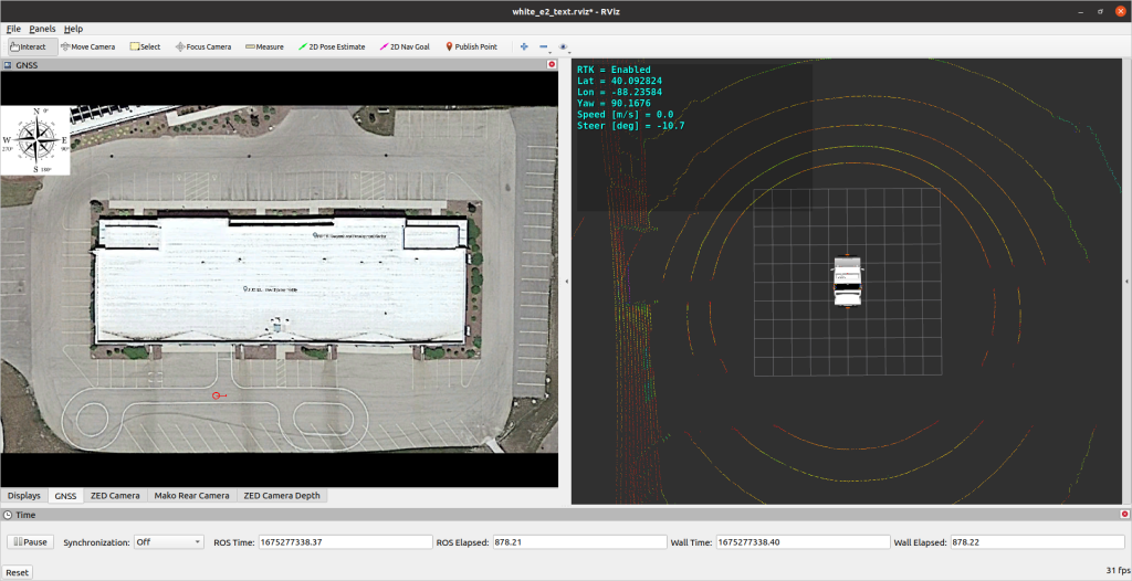
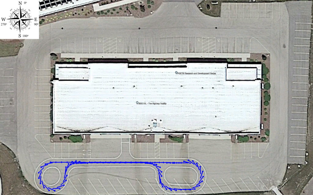
Demo
Stanley Lateral Controller (Kinematic/Dynamic Bicycle Model)
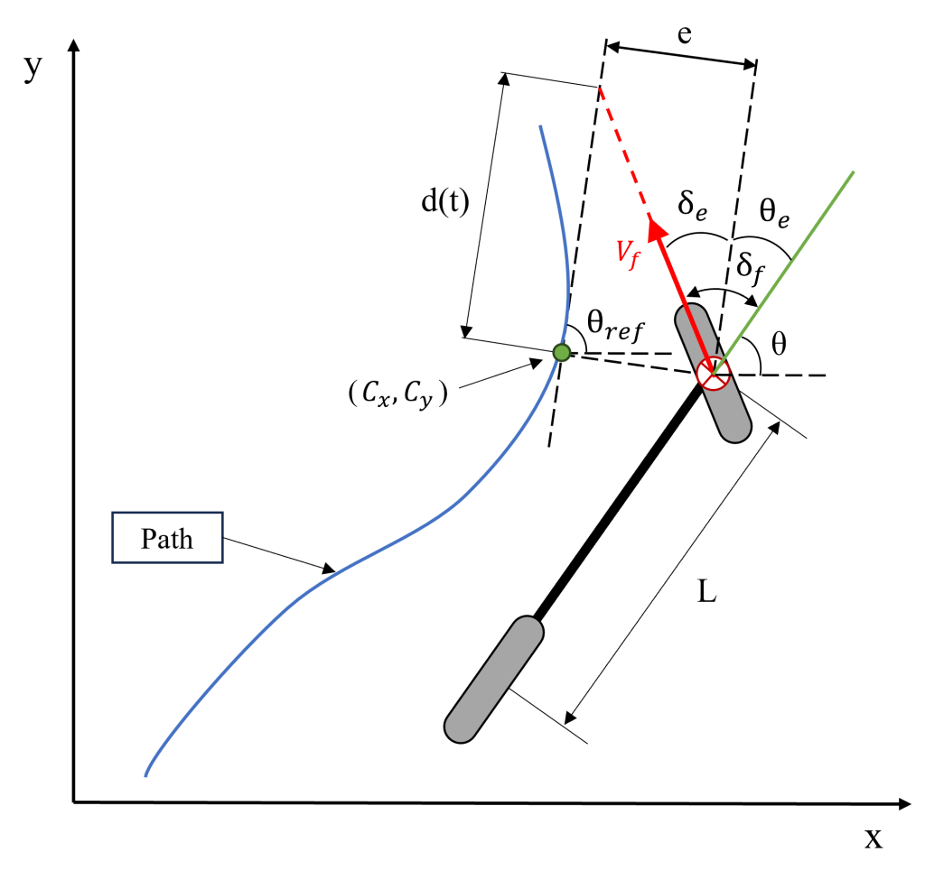
Stanley Controller Geometry

\(\theta\): heading of vehicle or yaw angle of vehicle
\(\dot{\theta}\): rotation rate of vehicle or yaw rate of vehicle
\(\theta_{e}\): heading error
\(\delta_f\): front steering angle, \(\delta_f \in [\delta_{min}, \delta_{max}]\)
\(L\): wheelbase
\(e\): crosstrack error
\(k\): controller gain
$$\dot e(t) \approx -k e(t) => e(t) = e(0)e^{-kt}$$ The error decays exponentially to 0. The decay rate is independent of vehicle speed and \(k\) is positive.
Recap: Stanley Controller Adjustment
Recap: Stanley Controller Summary
Demo


LQR Tracker with Feed Forward Term (Dynamic Bicycle Model)
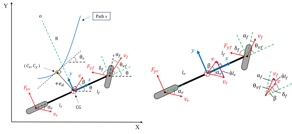
Dynamic Bicycle Model
\(\theta\): heading of vehicle or yaw angle of vehicle
\(v\) and \(a\): velocity of the center of mass and acceleration of center of mass
\(v_x\) and \(v_y\): longitudinal velocity and lateral velocity
\(a_x\) and \(a_y\): longitudinal acceleration and lateral acceleration, \(a_y = {v_x^2}/{R} = \kappa v_x^2\)
\(v_f\) and \(v_r\): velocity of front wheel and velocity of rear wheel
\(F_{yf}\) and \(F_{yr}\): lateral force of front/rear tire, \(F_{yf}=[2]C_{\alpha f}\alpha_f\), \(F_{yr}=[2]C_{\alpha r}\alpha_r\)
\(\alpha_f\) and \(\alpha_r\): slip angle of front/rear tire
\(C_{\alpha f}\) and \(C_{\alpha r}\): cornering stiffness of front/rear tire
\(l_f\) and \(l_r\): distance from front/rear wheel to the center of mass
\(\theta_{vf}\) and \(\theta_{vr}\): velocity angle of front/rear tire
\(\theta\): yaw angle in absolute coordinate
\(\beta\): slip angle of the center of mass in vehicle body coordinate
\(\theta+\beta\): heading angle in absolute coordinate
\(e_d\): lateral error, \(e_d\) is positive when road is on the left side of the vehicle
$$\sum F_y = m a_y = F_{yf}cos(\delta_f) + F_{yr}$$ $$\sum M = I \ddot{\theta} = F_{yf}cos(\delta_f) l_f – F_{yr} l_r$$ $$a_y = \frac{d^2y}{dt^2} = \ddot{y} + v_x\frac{v_x}{R}= \ddot{y} + v_x \dot{\theta} = \dot{v_y} + v_x \dot{\theta}$$ $$ma_y = C_{\alpha f}\alpha_f + C_{\alpha r}\alpha_r = m(\dot{v_y} + v_x \dot{\theta}) = C_{\alpha f} (\delta_f – \frac{\dot{\theta}l_f+v_y}{v_x}) + C_{\alpha r} (\frac{\dot{\theta}l_r-v_y}{v_x})$$ $$\dot{v_y} = \frac{C_{\alpha f}}{m} \delta_f + (\frac{C_{\alpha r} l_r – C_{\alpha f} l_f}{m v_x} – v_x)\dot{\theta} – \frac{C_{\alpha f} + C_{\alpha r}}{m v_x} v_y$$ $$\ddot{\theta} = \frac{C_{\alpha f} l_f}{I} \delta_f – \frac{C_{\alpha f} l_f^2 + C_{\alpha r} l_r^2}{I v_x} \dot{\theta} + \frac{C_{\alpha r} l_r – C_{\alpha f} l_f}{I v_x} v_y$$
Recap: Linearized Bicycle Dynamic Model$$ \begin{bmatrix} \ddot{y} \\ \ddot{\theta} \\ \end{bmatrix} = \begin{bmatrix} – \frac{C_{\alpha f} + C_{\alpha r}}{m v_x} & \frac{C_{\alpha r} l_r – C_{\alpha f} l_f}{m v_x} – {v_x} \\ \frac{C_{\alpha r} l_r – C_{\alpha f} l_f}{I v_x} & – \frac{C_{\alpha f} l_f^2 + C_{\alpha r} l_r^2}{I v_x} \\ \end{bmatrix} \begin{bmatrix} \dot{y} \\ \dot{\theta} \\ \end{bmatrix} % + % \begin{bmatrix} \frac{C_{\alpha f}}{m} \\ \frac{C_{\alpha f} l_f}{I} \\ \end{bmatrix} % \delta_f $$ $$ \begin{bmatrix} \dot{e}_d \\ \ddot{e}_d \\ \dot{e}_{\theta} \\ \ddot{e}_{\theta} \\ \end{bmatrix} = \begin{bmatrix} {0} & {1} & {0} & {0} \\ {0} & – \frac{C_{\alpha f} + C_{\alpha r}}{m v_x} & \frac{C_{\alpha f} + C_{\alpha r}}{m} & \frac{C_{\alpha r} l_r – C_{\alpha f} l_f}{m v_x} \\ {0} & {0} & {0} & {1} \\ {0} & \frac{C_{\alpha r} l_r – C_{\alpha f} l_f}{I v_x} & -\frac{C_{\alpha r} l_r – C_{\alpha f} l_f}{I} & – \frac{C_{\alpha f} l_f^2 + C_{\alpha r} l_r^2}{I v_x} \\ \end{bmatrix} \begin{bmatrix} {e}_d \\ \dot{e}_d \\ {e}_{\theta} \\ \dot{e}_{\theta} \\ \end{bmatrix} $$ $$ + % \begin{bmatrix} {0} \\ \frac{C_{\alpha f}}{m} \\ {0} \\ \frac{C_{\alpha f} l_f}{I} \\ \end{bmatrix} % \delta_f % + % \begin{bmatrix} {0} \\ \frac{C_{\alpha r} l_r – C_{\alpha f} l_f}{m v_x} – {v_x} \\ {0} \\ – \frac{C_{\alpha f} l_f^2 + C_{\alpha r} l_r^2}{I v_x} \\ \end{bmatrix} % \dot{\theta}_r $$ $$ \dot{X} = AX + B_1 \delta_f + B_2 \dot{\theta}_r \quad where \quad X = \begin{bmatrix} {e}_d \\ \dot{e}_d \\ {e}_{\theta} \\ \dot{e}_{\theta} \\ \end{bmatrix} $$
Recap: Discrete-time LQR
$$
J = \sum_{k=0}^{\infty} X^T[k] Q X[k] + u[k]^T R u[k] \quad w.r.t. \quad x[k+1] = A_dx[k]+B_du[k]
$$
where \(A_d = (I – \frac{Adt}{2})^{-1}(I + \frac{Adt}{2})\) and \(B_d = Bdt\)
Riccati Equation
$$
P_{k-1} = Q + A_d^TP_kA_d-A_d^TP_kB_d(R+B_d^TP_kB_d)^{-1}B_d^TP_kA_d
$$
Feed Forward Term
The state space model for the closed-loop system under state feedback
$$
\dot{X} = AX + B_1 \delta_f + B_2 \dot{\theta}_r = (A- B_1)K X + B_2 \dot{\theta}_r
$$
The closed-loop system with feedforward term \(\delta_{ff}\) can be written as
$$
\dot{X} = AX + B_1 \delta_f + B_2 \dot{\theta}_r = (A- B_1)K X + B_1\delta_{ff} + B_2 \dot{\theta}_r
$$
where \(u = \delta_f = -K_{1\times4}X_{4\times1} + \delta_{ff}\)
Lateral Control – LQR, Longitudinal Control – PID
Model Predictive Control (Dynamic Bicycle Model)
Pretest demoLateral Control & Longitudinal Control – MPC
Reference
[2] Hoffmann, Gabriel M., et al. “Autonomous automobile trajectory tracking for off-road driving: Controller design, experimental validation and racing.” 2007 American control conference. IEEE, 2007.
[3] Snider, Jarrod M. “Automatic steering methods for autonomous automobile path tracking.” Robotics Institute, Pittsburgh, PA, Tech. Rep. CMU-RITR-09-08 (2009).
Back to top of the page
